
A Formal (ε–δ) Definition of Limit
The intuitive idea “f(x) gets arbitrarily close to L as x approaches c” becomes precise with the ε–δ definition. This post states the definition carefully, explains each quantifier, and gives proof templates and worked examples so you can apply it with confidence.
The ε–δ Definition
Let \(f\) be defined on an open interval containing \(c\) (possibly not at \(c\) itself), and let \(L\) be a real number. We write
\(\displaystyle\lim_{x\to c} f(x)=L\)
if and only if
\(\text{for every }\varepsilon>0\ \text{there exists }\delta>0\ \text{such that if }0<|x-c|<\delta,\ \text{ then }|f(x)-L|<\varepsilon.\)
Two essential remarks
- The statement \(\displaystyle\lim_{x\to c}f(x)=L\) asserts both that the limit exists and that its value is \(L\).
- The function need not be defined at \(c\). Limits concern nearby values, not the value at the point.
How to Prove a Limit (ε–δ Checklist)
Template
- Start: Let \(\varepsilon>0\) be arbitrary.
- Algebra/estimate: Manipulate \(|f(x)-L|\) until it is bounded by a multiple of \(|x-c|\) plus controlled constants.
- Choose δ: Propose \(\delta=\delta(\varepsilon)\) so that \(|f(x)-L|<\varepsilon\) follows whenever \(|x-c|<\delta\). If needed, use \(\delta=\min\{\text{helpful bounds}\}\) to keep auxiliary terms bounded.
- Verify: Finish with a clean implication: if \(0<|x-c|<\delta\), then the required inequality holds.
Example 1 — Linear function
Prove \(\displaystyle\lim_{x\to c}(2x+3)=2c+3\).
Proof.
Let \(\varepsilon>0\). Then
\(|(2x+3)-(2c+3)|=2|x-c|\).
Choose
\(\delta=\displaystyle\frac{\varepsilon}{2}\).
If \(0<|x-c|<\delta\), then
\(|(2x+3)-(2c+3)|=2|x-c|<2\delta=\varepsilon\). QED.
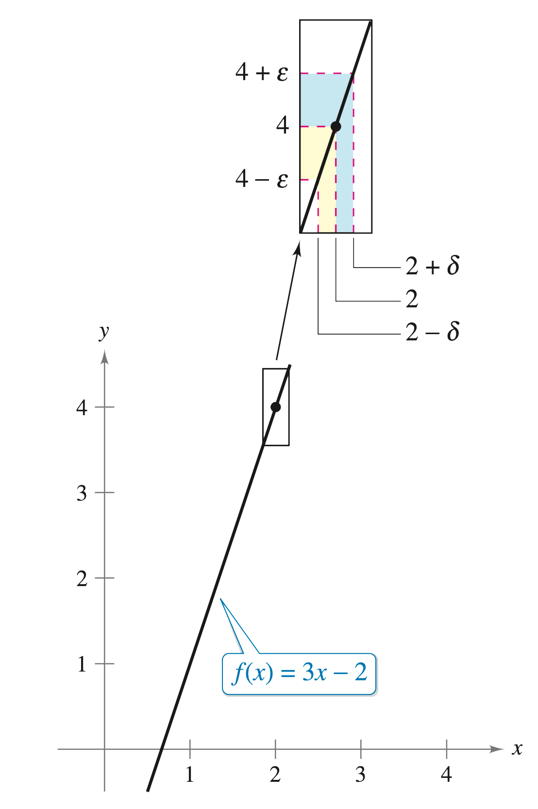
Example 2 — Prove a Limit Using the ε–δ Definition
Use the ε–δ definition of limit to prove that
\(\lim_{x \to 2}(3x – 2) = 4.\)
Proof.
You must show that for each \(\varepsilon > 0\), there exists a \(\delta > 0\) such that
\(\left|\left(3x – 2\right) – 4\right| < \varepsilon\)
whenever
\(0 < \left|x – 2\right| < \delta.\)
Because \(\delta\) depends on \(\varepsilon\), we look for a relation between
\(\left|\left(3x – 2\right) – 4\right| \quad \text{and} \quad \left|x – 2\right|.\)
We compute:
\(\left|\left(3x – 2\right) – 4\right| = \left|3x – 6\right| = 3\left|x – 2\right|.\)
So, for a given \(\varepsilon > 0\), choose
\(\delta = \frac{\varepsilon}{3}.\)
Then, whenever \(0 < \left|x – 2\right| < \delta\), we have
\(\left|\left(3x – 2\right) – 4\right| = 3\left|x – 2\right| < 3\left(\frac{\varepsilon}{3}\right) = \varepsilon.\)
Therefore,
\(\lim_{x \to 2}(3x – 2) = 4.\)
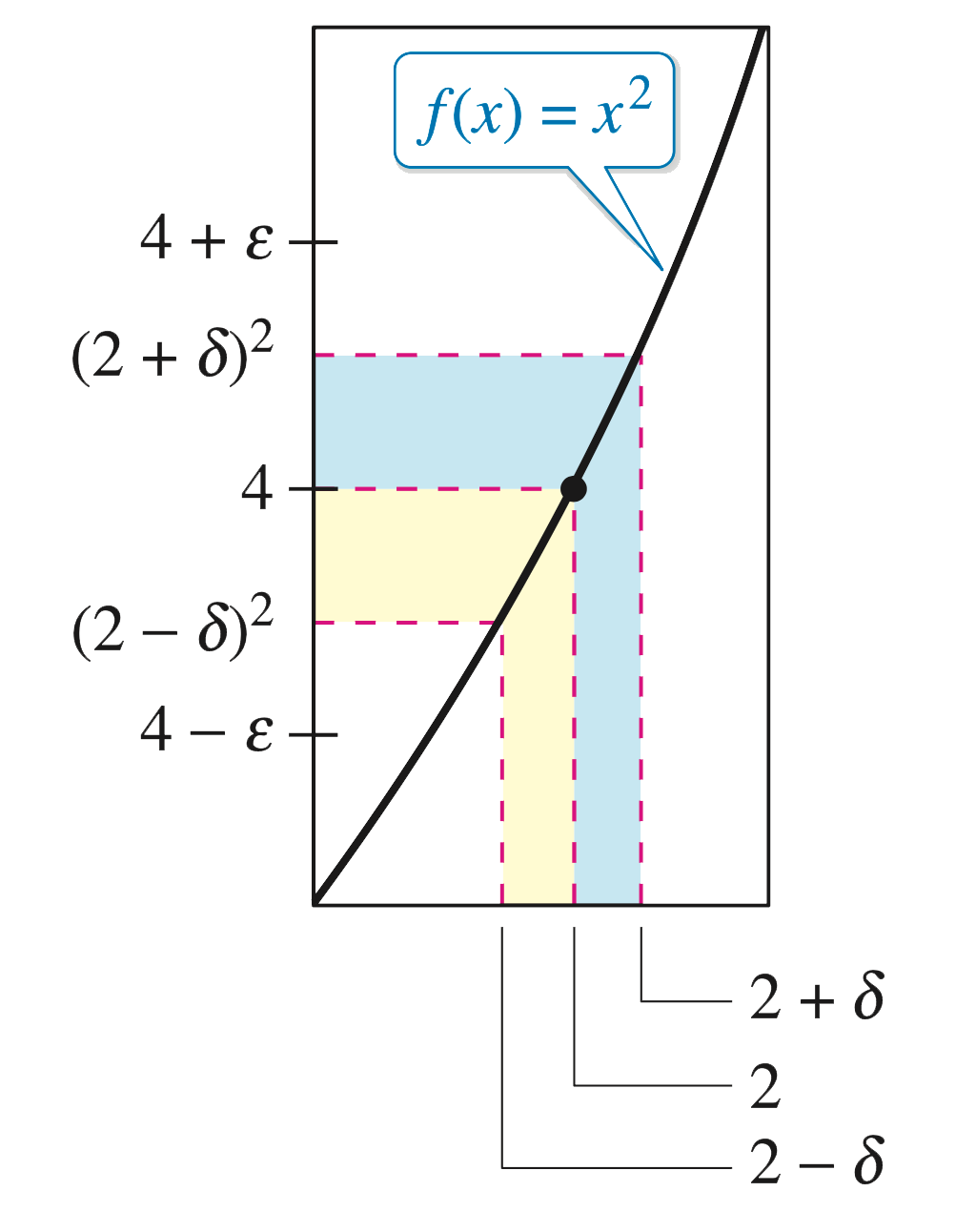
Example 3 — Quadratic Limit
Use the ε–δ definition of limit to prove that
\(\displaystyle \lim_{x \to 2}x^{2} = 4.\)
Proof.
You must show that for each \(\varepsilon > 0\), there exists a \(\delta > 0\) such that
\(\left|x^{2} – 4\right| < \varepsilon\)
whenever
\(0 < \left|x – 2\right| < \delta.\)
To find an appropriate \(\delta\), begin by writing
\(\left|x^{2} – 4\right| = \left|x – 2\right|\left|x + 2\right|.\)
For all \(x\) in the interval \(\left(1,3\right)\), we have \(x + 2 < 5\) and thus \(\left|x+2\right| < 5.\)
So, if we require \(\delta \leq 1\), then it follows that whenever
\(0 < \left|x – 2\right| < \delta\),
we get
\(\left|x^{2} – 4\right| = \left|x – 2\right|\left|x + 2\right| < \left(\frac{\varepsilon}{5}\right)\left(5\right) = \varepsilon.\)
As you can see, for \(x\)-values within \(\delta\) of 2 (\(x \neq 2\)), the values of \(f(x)\) are within \(\varepsilon\) of 4.
Uniqueness and Non-Existence
Uniqueness of limits
If both \(L_{1}\) and \(L_{2}\) satisfy the definition for \(\displaystyle\lim_{x\to c}f(x)\), then \(L_{1}=L_{2}\). Indeed, choose \(\varepsilon=\displaystyle\frac{|L_{1}-L_{2}|}{2}\) and apply each definition; the ε-balls do not overlap unless the centers coincide.
When a limit does not exist (DNE)
Consider \(f(x)=\begin{cases}1,& x\ge 0\\[2pt]0,& x<0\end{cases}\) at \(c=0\). The right-hand limit is 1 and the left-hand limit is 0, so no \(L\) can satisfy the ε–δ definition for all directions.
Practical Advice
Choosing δ effectively
- Try to bound “awkward” factors (like \(|x+c|\) or denominators) by forcing \(|x-c|<1\) first.
- When the bound is linear in \(|x-c|\), set \(\delta\) to a multiple of \(\varepsilon\). Otherwise, combine bounds with a minimum.
Common pitfalls
- Forgetting the condition \(0<|x-c|\) (we exclude the center point).
- Choosing \(\delta\) that does not depend on \(\varepsilon\) when the algebra clearly requires it.
- Using the value \(f(c)\) to justify a limit (irrelevant unless continuity is already known).
Summary
The ε–δ definition captures “approach” with complete precision: for each demanded output tolerance \(\varepsilon\), one can provide an input window \(\delta\) securing \(|f(x)-L|<\varepsilon\) whenever \(0<|x-c|<\delta\). Mastery comes from practicing the checklist, building estimates, and learning typical δ choices for linear, polynomial, rational, and trigonometric examples.
It’s Time to Practice!
Find the limit \(L\). Then use the ε–δ definition to prove that the limit is \(L\).
1. \(\displaystyle \lim_{x \to 4}\left(x + 2\right)\)
2. \(\displaystyle \lim_{x \to -2}\left(4x + 5\right)\)
3. \(\displaystyle \lim_{x \to -4}\left(\frac{1}{2}x – 1\right)\)
4. \(\displaystyle \lim_{x \to 3}\left(\frac{3}{4}x + 1\right)\)
5. \(\displaystyle \lim_{x \to 6} 3\)
6. \(\displaystyle \lim_{x \to 2}\left(-1\right)\)
7. \(\displaystyle \lim_{x \to 0}\sqrt[3]{x}\)
8. \(\displaystyle \lim_{x \to 4}\sqrt{x}\)
9. \(\displaystyle \lim_{x \to -5}\left|x – 5\right|\)
10. \(\displaystyle \lim_{x \to 3}\left|x – 3\right|\)
11. \(\displaystyle \lim_{x \to 1}\left(x^{2} + 1\right)\)
12. \(\displaystyle \lim_{x \to -4}\left(x^{2} + 4x\right)\)
13.
The statement
\(\displaystyle \lim_{x \to 2}\frac{x^{2} – 4}{x – 2} = 4\)
means that for each \(\varepsilon > 0\) there corresponds a \(\delta > 0\) such that if
\(0 < \left|x – 2\right| < \delta,\)
then
\(\left|\displaystyle\frac{x^{2} – 4}{x – 2} – 4\right| < \varepsilon.\)
If \(\varepsilon = 0.001\), then
\(\left|\displaystyle\frac{x^{2} – 4}{x – 2} – 4\right| < 0.001.\)
Use a graphing utility to graph each side of this inequality. Use the zoom feature to find an interval \(\left(2 – \delta,\ 2 + \delta\right)\) such that the graph of the left side is below the graph of the right side of the inequality.